Getting Started

To start using SPyCCI, you need a working Python installation together with the pip package manager. Officially supported Python versions are 3.10, 3.11, and 3.12. Python 3.13 is not yet officially supported, but no compatibility issues have been reported, and support is planned.

Tip: using a virtual environment

We always recommend installing new Python packages in a clean Conda environment and avoid installing in the system Python distribution or in the base Conda environment! If you are unfamiliar with Conda, please refer to their documentation for a guide on how to set up environments.

The SPyCCI package can be installed in two ways:

Installation from pip of a stable release
Download of the latest development version of the GitHub repository

Installing from pip

The SPyCCI package can be installed directly from pip using the command:

pip install spycci-toolkit

Installing the latest version from GitHub

The latest development version of SPyCCI can be installed by first downloading the repository from our GitHub page and then installing via pip. To do so, the following sequence of commands can be used:

git clone https://github.com/hbar-team/SPyCCI
cd SPyCCI
pip install .

If you intend to modify the library for development purposes, the library can be installed in editable mode using the command:

pip install -e .

More information about working on the library code and contributing to it’s GitHub repository are presented in the contributor’s guide.

Third party software compatibility

Being an interface package, SPyCCI requires the user to manually install all the required computational chemistry packages and made them available setting the proper environment variables. Not all the version of the sofwares are however fully compatible with SPyCCI. The following table lists all the supported software versions according to the following legend:

✅: full support, (recommended version)
☑️: full support
⚠️: partial support, some functionality may not be available
⛔: not supported or bugged

Software	Version	Support	Notes
Orca	6.x	✅
Orca	5.x	⚠️	Fully compatible with the exception of methods using the OpenCOSMO-RS model (introduced in 6.x)
Orca	4.x	⚠️	Some methods (like NEB-TS) may not be available
Orca	3.x	⛔	Incompatible due to different input file notation
xTB	6.7.1	⛔	See: https://github.com/crest-lab/crest/issues/357 and https://github.com/crest-lab/crest/issues/417
xTB	6.7.0	✅
xTB	6.6.x	☑️
xTB	6.4.x	☑️
crest	3.x	✅
crest	2.x	⚠️	Some methods may require the installation of additional software, see the crest manual for more details
DFTB+	24.1	✅
DFTB+	23.1	☑️

Versions different from those in the list are to be considered not ufficially supported.

Using the library

Once installed, the spycci-toolkit package can be accessed by the user and used in a common python script. The root of the package is simply named spycci so that the library can be imported simply using the syntax:

import spycci

Alternatively, individual submodules, classes, and functions can be imported separately using standard python syntax such as:

from spycci import systems
from spycci.engines import dftbplus
from spycci.wrappers.packmol import packmol_cube

For a more detailed explanation of the available features in each submodule, please refer to their specific page in the user guide.

Running a simple calculation

To familiarize on the basic usage of the library let us consider a simple ecample: the geometry optimisation of a water molecule. To do so, the first step is that of obtaining the initial geometrical structure of the system in the form of a .xyz file. You can obtain it from available databases, or you can draw the structures yourself in programs such as Avogadro.

Below is the water.xyz file, containing the structure of the water molecule, which we will use in these examples:

3

O   0.000  -0.736   0.000  
H   1.442   0.368   0.000  
H  -1.442   0.368   0.000  

If you open the file in a molecular visualization software, you will notice the structure is distorted from the typical equilibrium geometry. We can then optimise the structure by utilising one of the engines implemented in SPyCCI. We will use xTB in this example, due to its balance between accuracy and speed. The library needs the program to already be installed and ready to go. Let’s go through each step of the process together:

1) Importing the library

Before starting, we need to create a Python script and import the necessary classes from the library. We need the System class to store the information about our water molecule, and the XtbInput class to define the simulation setup (Hamiltonian, parameters, solvation, etc.):

from spycci.systems import System
from spycci import XtbInput  # Engines can also be imported directly from spycci 

2) Creating the System object

After importing the necessary modules, we can create our molecule, by indicating the (relative, or complete) path where the .xyz file is located:

water = System.from_xyz("example_files/water.xyz")

3) Creating a XtbInput object

We can now set up a engine object using an instance of XtbInput. Most of these engines come with sensible default options for calculations on small organic molecules in vacuum. To see all the available options, please refer to the engine section of the API documentation.

xtb = XtbInput()

4) Carrying out the calculation

We can now carry out the calculation. We want to do a geometry optimization on our water molecule, and we want the original information for the molecule to be updated after the calculation (inplace flag). The syntax for this calculation is as follows:

xtb.opt(water, inplace=True)

5) Printing the results

If you want to see the data currently stored in our System object, simply ask for it to be printed to screen:

print(water)

=========================================================
SYSTEM: water
=========================================================

Number of atoms: 3
Charge: 0
Spin multiplicity: 1

********************** GEOMETRY *************************

Total system mass: 18.0153 amu

----------------------------------------------
 index  atom    x (Å)      y (Å)      z (Å)   
----------------------------------------------
 0       O     0.03595    2.78898    0.00000  
 1       H     1.00595    2.78898    0.00000  
 2       H    -0.28738    2.19789    0.69783  
----------------------------------------------

********************** PROPERTIES *************************

Geometry level of theory: None
Electronic level of theory: None
Vibronic level of theory: None

Electronic energy: None Eh
Gibbs free energy correction G-E(el): None Eh
Gibbs free energy: None Eh
pKa: pKa object status is NOT SET

Et voilà! You have successfully carried out a geometry optimization for the water molecule using the SPyCCI library!

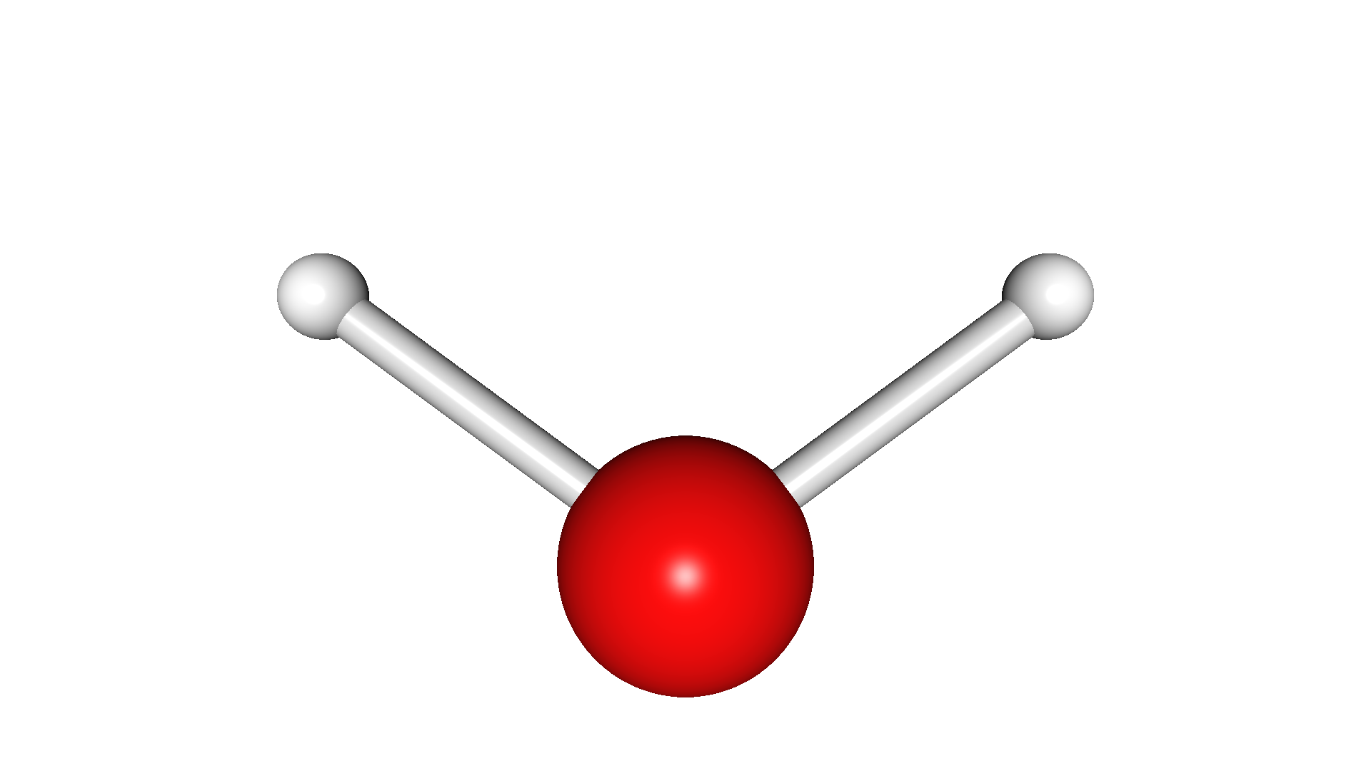
Basic molecule visualization

The SPyCCI library also offers simple tools to visualize the structure of the molecules encoded by a System object. As an example, the distorted structure of the input molecule, loaded into the water object, can be visualized using the built in mogli interface using the commands:

from spycci.tools.moglitools import MogliViewer

viewer = MogliViewer(water)
viewer.show()

The output image, freely capable of rotating, will look something like this: