Calculating properties
The spycci.functions submodule provides a suite of methods for calculating various physical properties of the system under investigation. These functions cover a broad range of topics and often perform multiple operations to assist users in computing chemically relevant results.
When working within the functions submodule, it is important for users to understand the implications of the calculations performed, including the underlying assumptions and approximations. As spycci.functions is continuously evolving, it offers workflows of both general applicability and more specialized use cases. Consequently, users are expected to have a solid understanding of each function’s structure and its required arguments.
Due to the complexity of many functions, they may perform only minimal sanity checks, relying on the user to ensure the accuracy and appropriateness of the input data. For instance, if a user calculates the pKa using a direct method with an unoptimized geometry, the result will reflect the properties of that unoptimized structure.
Empirical corrections
The functions to calculate pKa and reduction potentials take into account the self-energy of proton and electron for calculations carried out with GFN2-xTB:
electron self energy = \(111.75\, \mathrm{kcal/mol}\)
proton self energy = \(164.22\, \mathrm{kcal/mol}\)
pKa calculations
The spycci.functions.pka submodule provides an interface for the computation of the \(\mathrm{pKa}\) of a given species. The module is, at this time, composed by four functions:
calculate_pka: Computes the pKa of a molecular system using the direct scheme. The user must provide both the structures of the protomer \(HA\) and deprotomer \(A^-\) in the form ofSystemobjects with already optimized structures and defined electronic energy and possibly a vibronic one (see later the note about Vibrationless pKa calculations).calculate_pka_oxonium_scheme: Computes the pKa of a molecular system using the oxonium scheme. The user must provide the structures of the protomer \(HA\), deprotomer \(A^-\), water \(H_2O\) and oxonium ion \(H_3O^+\) in the form ofSystemobjects with already optimized structures and defined electronic energy and possibly a vibronic one (see later the note about Vibrationless pKa calculations).auto_calculate_pka: Computes the pKa of a given molecule by automatically searching the lowest-energy deprotomer using CREST. Once the proper deprotomer has been identified the function takes care of the geometry optimization of both structures, the calculation of electronic energies and frequencies (see later the note about Vibrationless pKa calculations). With the obtained result the pka is automatically computed using the direct scheme.run_pka_workflow: Given the protomer and deprotomer structures, the function takes care of the geometry optimization of both structures in solvent and the calculation of electronic energies and frequencies both in solvent and, if required, in vacuum. The function then computes the pka using both the direct and the oxonium schemes. If required the function computes also a pka using the COSMO-RS solvation energies using the oxonium scheme. Please notice how by running this workflow the frequency calculation cannot be skipped.
Vibrationless pKa calculations
The funtions calculate_pka, calculate_pka_oxonium_scheme and auto_calculate_pka allow the user to run a pKa calculation without running any frequency calculation. This is sometimes used in high-trhoughput settings but its not advisable for rigorous computational chemistry. Runnig these function without frequency calculations will subtitute the Gibbs free energy terms of each molecule involved with the corresponding electronic energies loosing all vibrational components and the free energy corrections.
The “direct” scheme
In the direct scheme, the pKa of a given molecule \(HA\) is computed considering the reaction scheme:
The equilibrium constant of the reaction is then computed as:
where:
where \(G_{aq}(A^{-})\), \(G_{aq}(H^{+})\) and \(G_{aq}(HA)\) represents the free energies of the molecules in acquous solution and the term \(RT \ln{(24.46)}\) corresponds to the free energy variation associated to the change in standard state with a concentration of \(1\mathrm{atm/l}\) for gas phase and \(1\mathrm{mol/l}\) for solution phase to a standard state with concentrations of \(1\mathrm{mol/l}\) for both the gas phase and solution [1].
In the direct scheme the free-energies \(G_{aq}(HA)\) and \(G_{aq}(A^{-})\), associated with the protomer and deprotomer, are/should be computed running optimization and frequency calculations in water solvent. The proton free energy in water \(G_{aq}(H^{+})\) is obtained from empyrical data. In SPyCCI the proton free energy in water plus the \(RT \ln{(24.46)}\) is assumed to be \(-270.29 \mathrm{kcal/mol}\) at \(298.15\mathrm{K}\).
The “oxonium” scheme
In the oxonium scheme the pKa of a given molecule \(HA\) is computed considering the following reaction scheme:
The equilibrium constant of such reaction can be related to the \(K_a\) according to:
or equivalently:
where, for the present scheme, \(\Delta G_{aq}\) can be obtained as:
where \(G_{aq}(A^{-})\), \(G_{aq}(H_3O^{+})\), \(G_{aq}(HA)\) and \(G_{aq}(H_2O)\) represents the free energies of the molecules in acquous solution. In the oxonium scheme all these quantities are computationally accessible and are/should be computed running optimization and frequency calculations in water solvent. The concentration of the water \([H_2O]\) is computed as the ratio of the water density of \(997 \mathrm{g/l}\) at \(25\mathrm{°C}\) and its molar mass of \(18.01528 \mathrm{g/mol}\).
The pka property structure
Given the peculiarity of the pKa calculation process and the variety of possible schemes employed, the pka property has been structured to give to the user the most clear picture possible of its origin and the involved approximations. To do so, the dedicated class object pKa has been defined.
The spyccy.core.properties.pKa class is a simple object collecting all the pka values computed according to different schemes (direct, oxonium and oxonium_cosmors), all the free energies used in the computation (free_energies) and, if used, the level of theory used in the COSMO-RS based calculations (level_of_theory_cosmors).
To access the pka computed with a given scheme, an instance of the pKa class can be interrogated directly using a syntax equivalent to that of a dictionary. The available keys are "direct", "oxonium" and "oxonium COSMO-RS". The key provided to access the data are case-insensitive (e.g. “direct” and “DIRECT” are both valid).Alternatively each property can be accessed directly as direct, oxonium or oxonium_cosmors property attributes. Be aware that these arguments, together with the level_of_theory_cosmors, are protected as read-only properties to prevent involuntary write operations.
If the user decides to manually set one of the pka values the syntax set_direct(user_value) or set_oxonium(user_value) must be used. The only difference is represented by the COSMO-RS related properties oxonium_cosmors and level_of_theory_cosmors that must be set simultaneously using the setter set_oxonium_cormors(user_value, engine).
The free_energies argument is less structured and has been thought more to be a human-readable way to access the free energy values used in the calculations. As such no read-only protection has been implemented and the argumnent can be accessed and edit as a regular class attribute.
The pka property
All the functions return the computed pKa values and set the pKa property (system.properties.pka) of the protonated system. The auto_calculate_pka also returns the deprotonated system.
The calculate_pka() function:
The calculate_pka function takes as arguments the following elements:
protonated(System): molecule in its protonated formdeprotonated(System): molecule in its deprotonated form
Please notice how both the protonated and deprotonated molecules must already be optimized (in water) and must posses a valid electronic energy value. If the vibronic energy is provided, its contribution is taken into account during the calculation.
An example script that can be used to compute the pKa of a molecule is provided in what follows:
from spycci.engines.xtb import XtbInput
from spycci.systems import System
from spycci.functions.pka import calculate_pka

protonated = System.from_xyz("protonated.xyz", charge=0, spin=1)
deprotonated = System.from_xyz("deprotonated.xyz", charge=-1, spin=1)

xtb = XtbInput(solvent="water")
xtb.opt(protonated, inplace=True)
xtb.opt(deprotonated, inplace=True)

pka = calculate_pka(protonated, deprotonated)
The computed pka value is returned as a pKa object (with only the direct property set). The function automatically sets the pka property of the protonated system accordingly. If this is not desired, the feature can be decativated using the keyword only_return=True.
The calculate_pka_oxonium_scheme() function:
The calculate_pka_oxonium_scheme function takes as arguments the following elements:
protonated(System): molecule in its protonated formdeprotonated(System): molecule in its deprotonated formwater(System): the water moleculeoxonium(System): the oxonium ion molecule
Please notice how both the protonated and deprotonated molecules must already be optimized (in water) and must posses a valid electronic energy value. If the vibronic energy is provided, its contribution is taken into account during the calculation.
An example script that can be used to compute the pKa of a molecule is provided in what follows:
from spycci.engines.xtb import XtbInput
from spycci.systems import System
from spycci.functions.pka import calculate_pka_oxonium_scheme

protonated = System("protonated.xyz", charge=0, spin=1)
deprotonated = System("deprotonated.xyz", charge=-1, spin=1)
water = System("water.xyz", charge=0, spin=1)
oxonium = System("oxonium.xyz", charge=-1, spin=1)

xtb = XtbInput(solvent="water")
xtb.opt(protonated, inplace=True)
xtb.opt(deprotonated, inplace=True)
xtb.opt(water, inplace=True)
xtb.opt(oxonium, inplace=True)

pka = calculate_pka_oxonium_scheme(protonated, deprotonated, water, oxonium)
Please notice how the water and oxonium structures can either be entered manually by the user or retrived by the buit-in retrieve_structure helper function. The syntax of the previous scheme, in the second case, becomes:
from spycci.engines.xtb import XtbInput
from spycci.systems import System
from spycci.functions.pka import calculate_pka_oxonium_scheme
from spycci.functions.utils import retrieve_structure

protonated = System("protonated.xyz", charge=0, spin=1)
deprotonated = System("deprotonated.xyz", charge=-1, spin=1)

water_xyz = retrieve_structure("water")
water = System("water", charge=0, spin=1, geometry=water_xyz)

oxonium_xyz = retrieve_structure("oxonium")
oxonium = System("oxonium", charge=1, spin=1, geometry=oxonium_xyz)

xtb = XtbInput(solvent="water")
xtb.opt(protonated, inplace=True)
xtb.opt(deprotonated, inplace=True)
xtb.opt(water, inplace=True)
xtb.opt(oxonium, inplace=True)

pka = calculate_pka_oxonium_scheme(protonated, deprotonated, water, oxonium)
The computed pka value is returned as a pKa object (with only the oxonium property set). The function automatically sets the pka property of the protonated system accordingly. If this is not desired, the feature can be decativated using the keyword only_return=True.
The run_pka_workflow() function:
The run_pka_workflow function, takes as arguments the protomer and deprotomer structures (in the form of System objects).
The function takes care of the geometry optimization of both structures in solvent and the calculation of electronic energies and frequencies both in solvent and, if required, in vacuum. The level of theory of each calculation can be set using the method_geometry, method_electonic, method_vibrational keywords. Once all the calculations have been executed, the function then computes the pka using both the direct and the oxonium schemes. If required the function computes also a pka using the COSMO-RS solvation energies using the oxonium scheme. The routine takes as arguments the following elements:
protonated(System): The protonated system for which the pKa must be computeddeprotonated(System): The deprotomer generated during the dissociation reactionmethod_vibrational(XtbInputorOrcaInput): The engine to be used to run the frequency calculations.method_electonic(XtbInputorOrcaInput): The engine to be used to run the electronic calculations. If set toNone(default) will use electronic energy computed by themethod_vibrationalengine. Please notice that, if the electronic method is different from the vibrational one, the computed Gibbs Free energy will be a mix of two different levels of theory (not advaisable)method_geometry(XtbInputorOrcaInput): The engine to be used to run the geometry optimizations. If set toNonethe user-provided geometries will be use directly without optimization while the water molecule and oxonium ion structures will be otimized using the BP86/def2-TZVPD (as the default OpenCOSMO-RS settings).use_cosmors(bool): If set toTruewill also use OpenCOSMO-RS to compute solvation energies.use_engine_settings(bool): If set toTruewill use the engine level of theory to run the COSMO-RS calculation (not advisable) else the default BP86/def2-TZVPD level of theory will be used.ncores(Optional[int]): The number of cores to be used in the calculations. If set toNone(default) will use the maximun number of available cores.maxcore(Optional[int]): For the engines that supprots it, the memory assigned to each core used in the computation.
An example script that can be used to compute the pKa of a molecule is provided in what follows:
from spycci.engines.xtb import XtbInput
from spycci.engines.orca import OrcaInput
from spycci.systems import System
from spycci.functions.pka import run_pka_workflow

protonated = System("protonated.xyz", charge=0, spin=1)
deprotonated = System("deprotonated.xyz", charge=-1, spin=1)

xtb = XtbInput(solvent="water")
orca = OrcaInput(method="BP86", basis_set="def2-TZVPD", solvent="water")

pka, optimized_protonated = run_pka_workflow(
  protonated,
  deprotonated,
  method_vibrational = xtb,
  method_electonic = orca,
  method_geometry = xtb,
  use_cosmors = True,
  )
The computed pka value is returned as a pKa object together with the structure of the protonated molecule optimized in solvent (optimized_protonated). Please notice how the pka object in this case is NOT set in the protonated object properties but rather in the optimized_protonated system since it is referred to the optimized molecular structure that can differ from the input one. BEWARE that this behavior is conserved also in the method_geometry = None use case.
The auto_calculate_pka() function:
The auto_calculate_pka function takes as main argument the protonated molecule structure (in the form of a System object). The molecule is sequentially deprotonated using the CREST deprotomer search routine until the lowest energy deprotomer is identified. Once the deprotomer search has been completed, the structure of both molecules is optimized using the specified level of theory and both electronic and vibronic energies are computed at the user defined level of theory. The routine takes as arguments the following elements:
protonated(System): The protonated molecule for which the pKa must be computed.method_el(Engine): The computational engine to be used in the electronic level of theory calculations.method_vib(Engine): The computational engine to be used in the vibronic level of theory calculations. (optional)method_opt(Engine): The computational engine to be used in the geometry optimization of the protonated molecule and its deprotomers. (optional)ncores(int): The number of cores to be used in the calculations. (optional)maxcore(int): For the engines that supprots it, the memory assigned to each core used in the computation. (optional)
An example script that can be used to compute the pKa of a molecule is provided in what follows:
from spycci.engines.xtb import XtbInput
from spycci.systems import System
from spycci.functions.pka import calculate_pka

protonated = System.from_xyz(f"protonated.xyz", charge=0, spin=1)
xtb = XtbInput(solvent="water")

pka, deprotonated = auto_calculate_pka(
    protonated,
    method_el=xtb,
    method_vib=xtb,
    method_opt=xtb,
)
Please notice how the optimized structure of the deprotonated system is also returned together with the pKa value.
1-el redox potential
Calculates the one-electron reduction potential of a molecule \(MH_{n}\), considering a generic reaction of the type:
provided the following arguments:
oxidised(System): molecule in its oxidised statereduced(System): molecule in its reduced statepH(float, default:7.0): pH at which the reduction potential is calculated
and returns the reduction potential of the molecule considering the provided states at the provided pH, including eventual PCET mechanisms, calculated as:
where \(G_{M^{\cdot(n-1)-}}\) and \(G_{MH_{n}}\) are calculated summing the electronic + vibronic energies at the selected level of theory, \(G_{H^{+}} = -270.29 kcal/mol\), \(F = 23.061 kcal/volt–gram-equivalent\), and \(E_{SHE} = 4.28 V\).
Fukui functions
The spycci.functions.calculate_fukui function calculates the Fukui functions \(f^+(r)\), \(f^-(r)\) and \(f^0(r)\) associated with a given molecular geometry. The Fukui functions are computed according to the definitions:
Where, given a molecule with \(N\) electrons, \(\rho_{N}(r)\) represents its electronic density while \(\rho_{N\pm1}(r)\) represents the electronic density of the molecule, in the same nuclear configuration, when one electron is either added (\(+1\)) or removed (\(-1\)).
The Fukui functions are both computed as volumetric quantities and saved in a Gaussian Cube compatible format in the output_density folder and as condensed values saved in the System object properties attribute in the form of a dictionary. The condensed Fukui functions are computed by applying the \(f^+\), \(f^-\) and \(f^0\) definitions replacing the charge density with either the Mulliken charges or the Hirshfeld charges (changing the sign accordingly given that a localized electronic density represents an accumulation of electrons hence of negative charge). Please notice how the Hirshfeld charges are supported only by the OrcaInput engine.
Important
Please notice how the Fukui cubes contain the localized Mulliken-charge-based Fukui values in place of the atomic charges. This is explained in the first comment line of each cube file and, for sake of clarity, all the files are saved using the extension .fukui.cube.
The function can be called with the following minimal arguments:
molecule(System): The molecular structure to be used in the computationengine(OrcaInputorXtbInput): The engine defining the level of theory to be used in the calculation.
The function assumes that the molecule supports only singlet and doublet states and switches the spin multeplicity according to the number of electrons. If different spin states needs to be considered the spins_states option can be used to provide the spin multeplicity values as a list.
An example code snippet is provided in what follows:
from spycci.systems import System
from spycci.engines.orca import OrcaInput
from spycci.functions.fukui import calculate_fukui, CubeGrids

mol = System.from_xyz("./acetaldehyde.xyz")
orca = OrcaInput(method="PBE", basis_set="def2-SVP")

orca.opt(mol, inplace=True)
calculate_fukui(mol, orca, cube_grid=CubeGrids.FINE)

print(mol)
That for the acetaldehyde molecule returns the following result:
=========================================================
SYSTEM: acetaldehyde
=========================================================

Number of atoms: 7
Charge: 0
Spin multiplicity: 1

********************** GEOMETRY *************************

Total system mass: 44.0526 amu

----------------------------------------------
 index  atom    x (Å)      y (Å)      z (Å)
----------------------------------------------
 0       C    -3.00790    0.17495    0.13810
 1       C    -3.66800    1.53034    0.11359
 2       H    -3.22195    2.19896    0.87341
 3       H    -4.75895    1.41874    0.29379
 4       H    -3.56793    1.97830   -0.89850
 5       O    -2.11052   -0.15105    0.88722
 6       H    -3.42225   -0.55833   -0.62459
----------------------------------------------

********************** PROPERTIES *************************

Geometry level of theory: OrcaInput || method: PBE | basis: def2-SVP | solvent: None
Electronic level of theory: OrcaInput || method: PBE | basis: def2-SVP | solvent: None
Vibronic level of theory: OrcaInput || method: PBE | basis: def2-SVP | solvent: None

Electronic energy: -153.528266323306 Eh
Gibbs free energy correction G-E(el): 0.02861407 Eh
Gibbs free energy: -153.499652253306 Eh
pKa: pKa object status is NOT SET


MULLIKEN ANALYSIS
----------------------------------------------
 index  atom   charge    spin
----------------------------------------------
 0       C    0.05436   0.00000
 1       C    -0.04823  0.00000
 2       H    0.05176   0.00000
 3       H    0.05695   0.00000
 4       H    0.05677   0.00000
 5       O    -0.17156  0.00000
 6       H    -0.00005  0.00000

CONDENSED FUKUI - MULLIKEN
----------------------------------------------
 index  atom    f+      f-      f0
----------------------------------------------
 0       C    0.23610   0.08077   0.15843
 1       C    -0.11416  -0.02731  -0.07074
 2       H    0.12882   0.11125   0.12003
 3       H    0.15563   0.12121   0.13842
 4       H    0.15492   0.12121   0.13806
 5       O    0.22073   0.35571   0.28822
 6       H    0.21797   0.23717   0.22757

HIRSHFELD ANALYSIS
----------------------------------------------
 index  atom   charge    spin
----------------------------------------------
 0       C    0.14702   0.00000
 1       C    -0.07279  0.00000
 2       H    0.04088   0.00000
 3       H    0.04575   0.00000
 4       H    0.04567   0.00000
 5       O    -0.22623  0.00000
 6       H    0.01970   0.00000

CONDENSED FUKUI - HIRSHFELD
----------------------------------------------
 index  atom    f+      f-      f0
----------------------------------------------
 0       C    0.28818   0.15946   0.22382
 1       C    0.07190   0.09734   0.08462
 2       H    0.05820   0.06063   0.05941
 3       H    0.09907   0.07355   0.08631
 4       H    0.09850   0.07352   0.08601
 5       O    0.25823   0.37205   0.31514
 6       H    0.12592   0.16345   0.14468
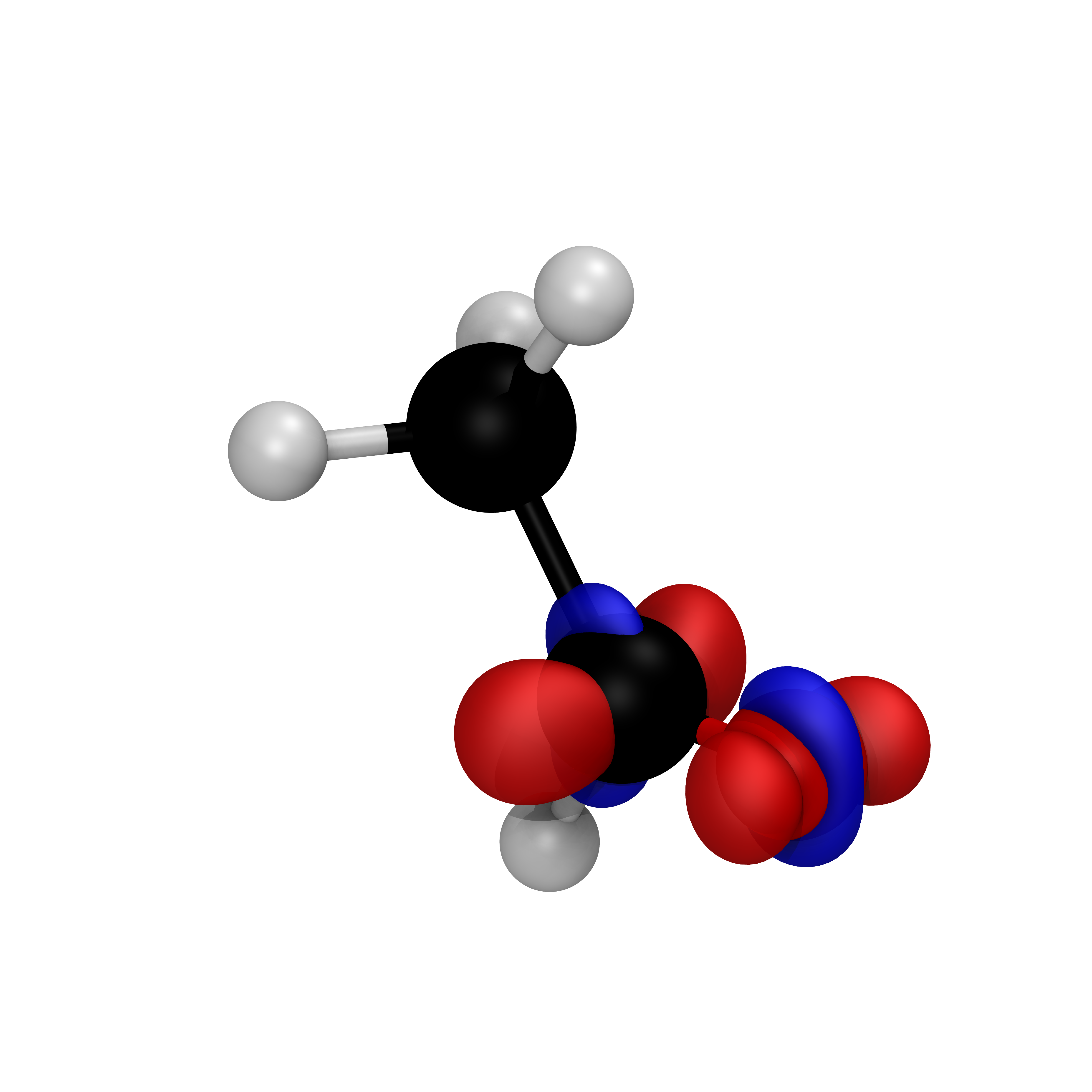
The volumetric fukui functions can then be plotted using the built in vmd based rendering tool. As an example the following code can be used to render the the \(f^+(r)\) Fukui function.
from spycci.tools.vmdtools import VMDRenderer

renderer = VMDRenderer(resolution=1200)
renderer.scale = 1.1

renderer.render_fukui_cube(
    "./output_densities/acetaldehyde_orca_PBE_def2-SVP_vacuum_Fukui_plus.fukui.cube",
    isovalue=0.02,
    show_negative=True
)
The rendered volume is saved in a .bmp bitmap image format. In the case of the acetaldehyde molecule considered in the example, the following image is obtained: