Molecular visualization using VMD
Beyond allowing the user to run computational chemistry calculations, the SPyCCI package also provides a simple interface to the Visual Molecular Dynamics (VMD) software enabling the user to render molecular structures and cube files directly from a python script. The interface is constantly updated with new features and, at the moment, supports the rendering of both molecular structures, provided either in the form of System objects, .xyz or pdb files, and volumetric data in the form of .cube files or Cube objects.
The core of the interface is represented by the VMDRenderer class. The class represents a generic rendering tool that can be created setting a resolution value, system position, orientation and zoom, graphical effects such as shadows, ambientocclusion and depth of field (DoF). Once created the class provides specific methods capable of generating the required renders.
Notes about cube files
The .cube format processed by SPyCCI is the Gaussian cube file format. The file is composed by a header and a body of volumetric data. The header is structured as:
Two comment lines.
A line listing the number of atoms included in the file followed by the position of the origin of the volumetric data.
Three lines listing the number of voxels along each axis (
x,y,z) followed by the axis vector. The length of each vector is the length of the side of the voxel thus allowing non cubic volumes. If the sign of the number of voxels in a dimension is positive then the units are Bohr, if negative then Angstroms.A section with a number of lines equal to the number of atoms in the molecule and consisting of 5 numbers: the first is the atom number, the second is the charge (this field is often used for other data types), and the last three are the
x,y,zcoordinates of the atom center.
The body of volumetric data is represented by a series of lines listing floating point values for each voxel. The data is usually arranged in columns of 6 values generated by looping on the voxel coordinates with x axis as the outer loop and z as the most inner one.
Rendering a molecule from a .xyz file
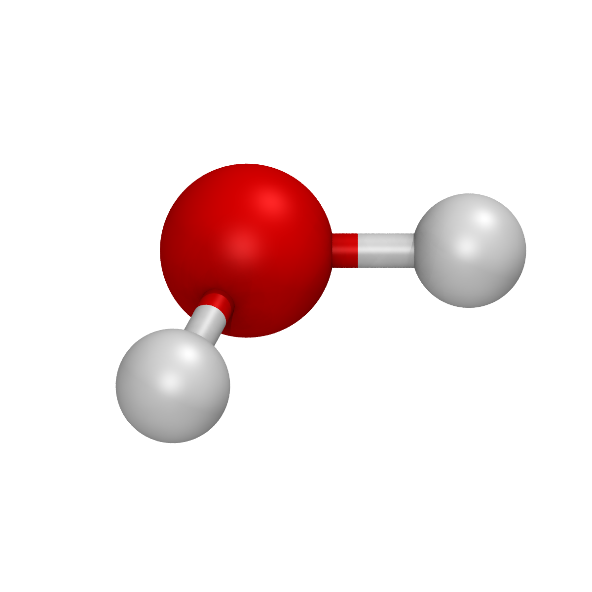
The structure of a molecule can be rendered starting from a .xyz file by using the render_system_file() function. As an example, the following script can be used to render a simple water.xyz file:
from spycci.tools.vmdtools import VMDRenderer

vmd = VMDRenderer(resolution=1200)
vmd.render_system_file("./water.xyz")
This will save a water.bmp image file that looks like this:
Rendering a molecule from a System object
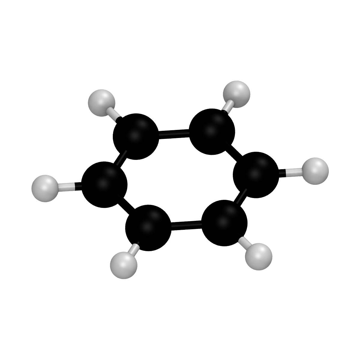
Similarly from what shown in the case of a .xyz file, the VMDRenderer class directly supports the rendering of System objects. This can be done using the render_system() function. As an example, the following script can be used to render a benzene molecule generated from its SMILES string:
from spycci.systems import System
from spycci.tools.vmdtools import VMDRenderer

mol = System.from_smiles("benzene", "c1ccccc1")

renderer = VMDRenderer(resolution=1200)
renderer.scale = 1.5
renderer.xyx_rotation = [-45., 0., 0.]

renderer.render_system(mol)
Please notice how the scale argument has been set to 1.5 to zoom while a rotation of 45° has been applied to the x axis. The output of such a script is a benzene_0_1.bmp file:
Notes about rotations
The current implementation of the VMDRendered class uses an XYX rotation sequence, following the convention of proper Euler angles. Unlike intrinsic rotations tied to the molecular frame, these rotations are applied around the camera (screen) axes, which change orientation after each step. As a result, the second application of the X-axis rotation occurs around a different orientation than the first, due to the intermediate Y-axis rotation. This sequence allows representation of arbitrary 3D orientations, despite the repeated axis label.
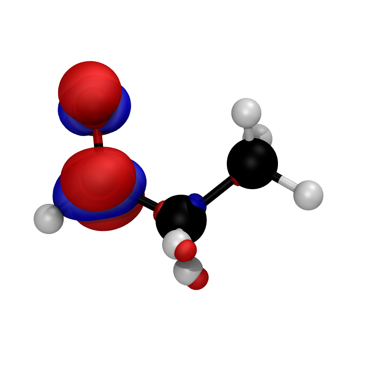
Rendering a generic .cube file
Rendering of a generic cube file can be achieved using the render_cube_file() function of the VMDRenderer class. The function, that can be called by simply providing the name of the cube file, can be set to render positive and negative regions of volumetric data with a user specified isovalue. If the isovalue is not explicilty indicated a default value will be computed as the 20% of the maximum voxel value (in absolute values). Additional features such as the color of the positive and negative reagions, whether to show the negative part of the cube or the filename of the output file, can be set by the user using the built in keywords.
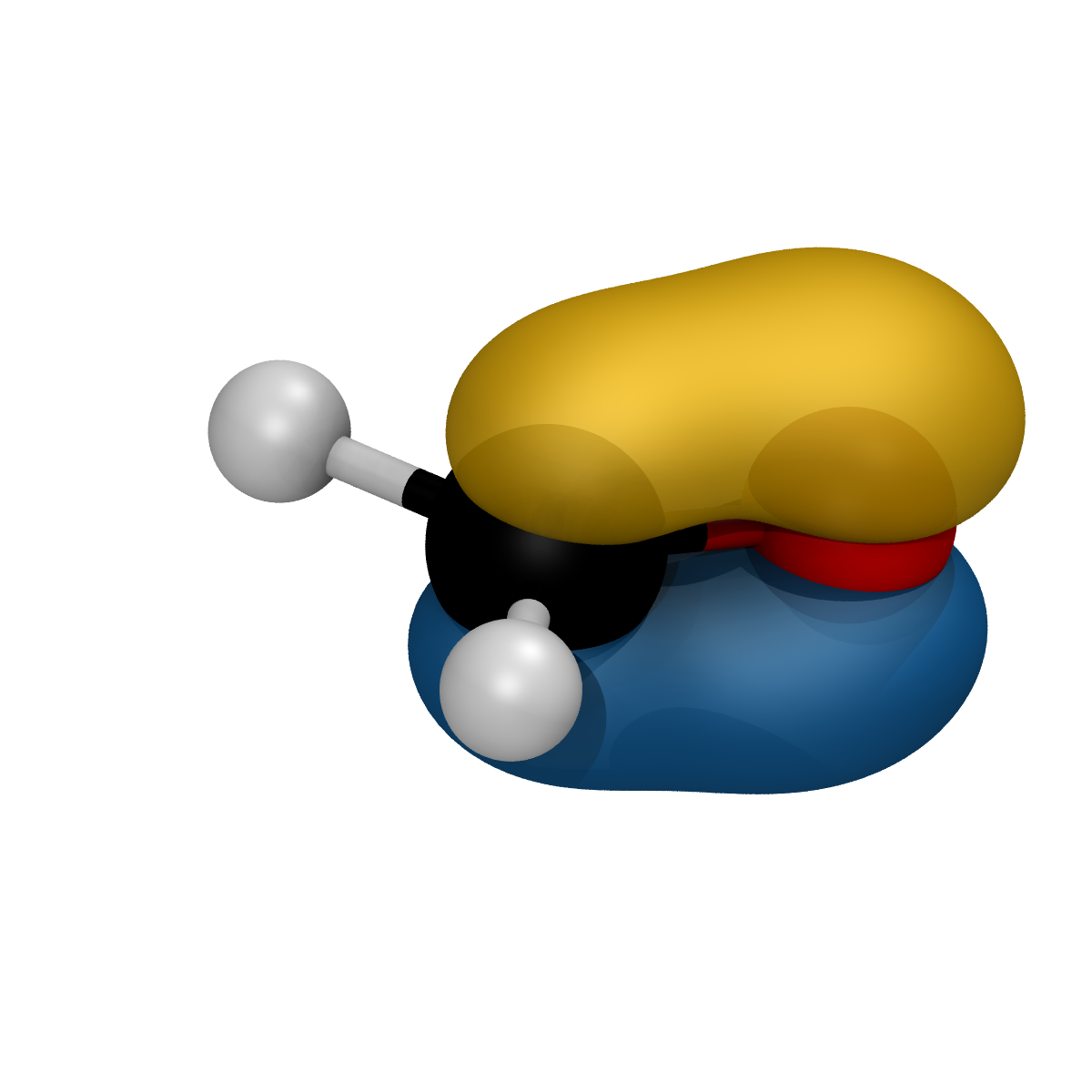
As an example, the 6th molecular orbital for the formaldehyde molecule, generated by orca as a input.mo6a.cube file. Can be simply rendered using the code:
from spycci.tools.vmdtools import VMDRenderer

renderer = VMDRenderer(resolution=1200)
renderer.scale = 1.0
renderer.xyx_rotation = [120.0, 20.0, 0.0]

renderer.render_cube_file(
    f"./input.mo6a.cube",
    positive_color=32,
    negative_color=23,
    show_negative=True,
)
resulting in the following input.mo6a.bmp image file:
Notes about ORCA’s molecular orbitals (MOs) cube files
The cube files generated by ORCA when exporting molecular orbitals differs from the standard structure of the Gaussian cube file format. The number of atoms is represented by a negative number and an additional line is added after the atoms coordinates section. The differences in formatting are taken into account by SPyCCI that automatically converts this format to a regular Gaussian cube for visualization with vmd.
Rendering volumetric data from a Cube object
Similarly from what shown in the case of a .cube file, the VMDRenderer class directly supports the rendering of Cube objects. This can be done using the render_cube() function in complete analogy with the syntax discussed before for the render_cube_file() function. The only difference in this case is the requirement for the user to provide a filename since, differently from what seen in the case of a System object, a Cube object has not assigned name.
As an example, the previous example about plotting the 6th molecular orbital of the formaldehyde molecule from a input.mo6a.cube cube file can be revritten as follows:
from spycci.tools.cubetools import Cube
from spycci.tools.vmdtools import VMDRenderer

renderer = VMDRenderer(resolution=400)
renderer.scale = 1.0
renderer.xyx_rotation = [120.0, 20.0, 0.0]

cube = Cube.from_file("./input.mo6a.cube")

renderer.render_cube(
    cube,
    f"./formaldehyde_MO6a.bmp",
    positive_color=32,
    negative_color=23,
    show_negative=True,
)
This will generate a formaldehyde_MO6a.bmp file identical to the one shown in the previous example.
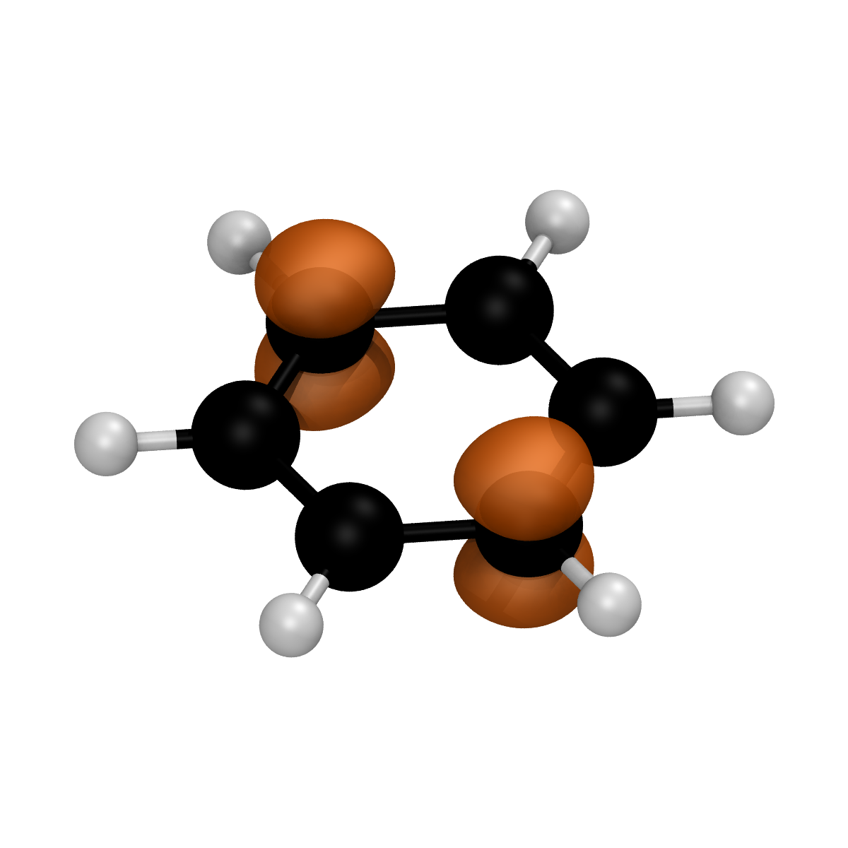
Rendering an ORCA spin density (.spindens.cube) file
A spin density cube generated from orca (having the .spindens.cube extension) can be rendered using the dedicated render_spin_density_cube() function. In the following simple example, the spin density obtained form a DFT calculation has been saved and directly rendered from the output_densities folder:
from spycci.systems import System
from spycci.engines.orca import OrcaInput
from spycci.tools.vmdtools import VMDRenderer

mol = System.from_smiles("benzene", "c1ccccc1", charge=1, spin=2)

orca = OrcaInput(method="B3LYP", basis_set="def2-TZVP", ncores=4)
orca.spe(mol, save_cubes=True, inplace=True)

renderer = VMDRenderer(resolution=1200)
renderer.scale = 1.5
renderer.xyx_rotation = [-45.0, 0.0, 0.0]

renderer.render_spin_density_cube(
    "./output_densities/benzene_1_2_orca_B3LYP_def2-TZVP_vacuum_spe.spindens.cube",
    filename="spindensity.bmp"
)
The result is a spindensity.bmp (the name of the output has been manually set using the filename option):
Rendering an Fukui functions (.fukui.cube) file
Volumetric maps of Fukui functions generated from the SPyCCI calculate_fukui() function, and saved in cube format (having the .fukui.cube extension), can be rendered using the dedicated render_fukui_cube() function. In the following simple example, the Fukui \(f^+(r)\) function obtained form a DFT calculation on the propionaldehyde molecule has been saved and directly rendered from the output_densities folder:
from spycci.systems import System
rom spycci.engines.xtb import XtbInput
from spycci.engines.orca import OrcaInput
from spycci.functions.fukui import calculate_fukui, CubeGrids

from spycci.tools.vmdtools import VMDRenderer

mol = System.from_smiles("propionaldehyde", "CCC=O")
xtb = XtbInput()

xtb.opt(mol)

orca = OrcaInput(method="PBE", basis_set="def2-SVP", ncores=4)
calculate_fukui(mol, orca, cube_grid=CubeGrids.FINE)

renderer = VMDRenderer(resolution=1200)
renderer.scale = 1.4
renderer.xyx_rotation = [-100.0, 180.0, 90.0]

renderer.render_fukui_cube(
    "./output_densities/propionaldehyde_orca_PBE_def2-SVP_vacuum_Fukui_plus.fukui.cube",
    isovalue=0.01,
    show_negative=True,
    filename="fukui_plus.bmp",
)
The output of the renderer call is a fukui_plus.bmp image file:
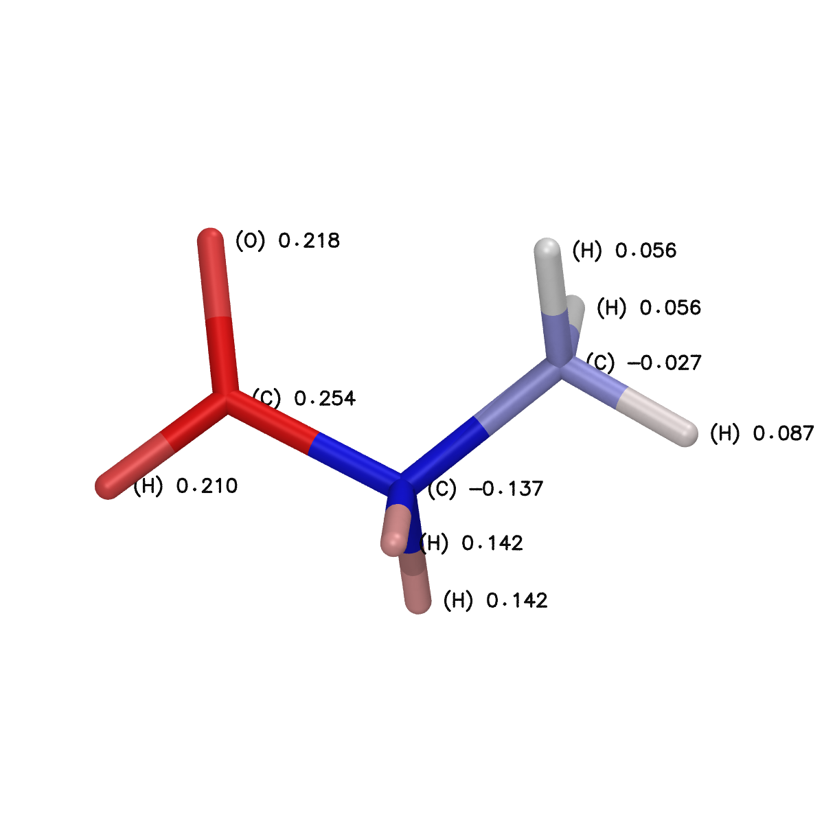
Similarly condensed Fukui values, saved in the charge column of the .fukui.cube file, can be rendered using the render_condensed_fukui() function according to the syntax:
renderer.render_condensed_fukui(
    "./output_densities/propionaldehyde_orca_PBE_def2-SVP_vacuum_Fukui_plus.fukui.cube",
    filename="condensed_fukui_plus.bmp",
)
that outputs the following condensed_fukui_plus.bmp image file: